CAIIB ABFM Module B — Working Capital Management Deep Dive

Working capital is what keeps the lights on at every operating business — and Module B of the CAIIB ABFM (Advanced Business & Financial Management) paper devotes the bulk of its mark weight to teaching bankers how to assess, structure, and monitor it. Understand working capital management deeply and you're not only acing this section of ABFM, you're also doing the daily job of credit appraisal more skilfully than 80% of your peers.

This article walks through the working-capital management content in ABFM Module B in working-banker language: the operating cycle, working-capital gap, the MPBF and Turnover methods, cash conversion cycle, and the inventory / receivables / cash management techniques that show up in IIBF exam papers.

The operating cycle — the foundation concept

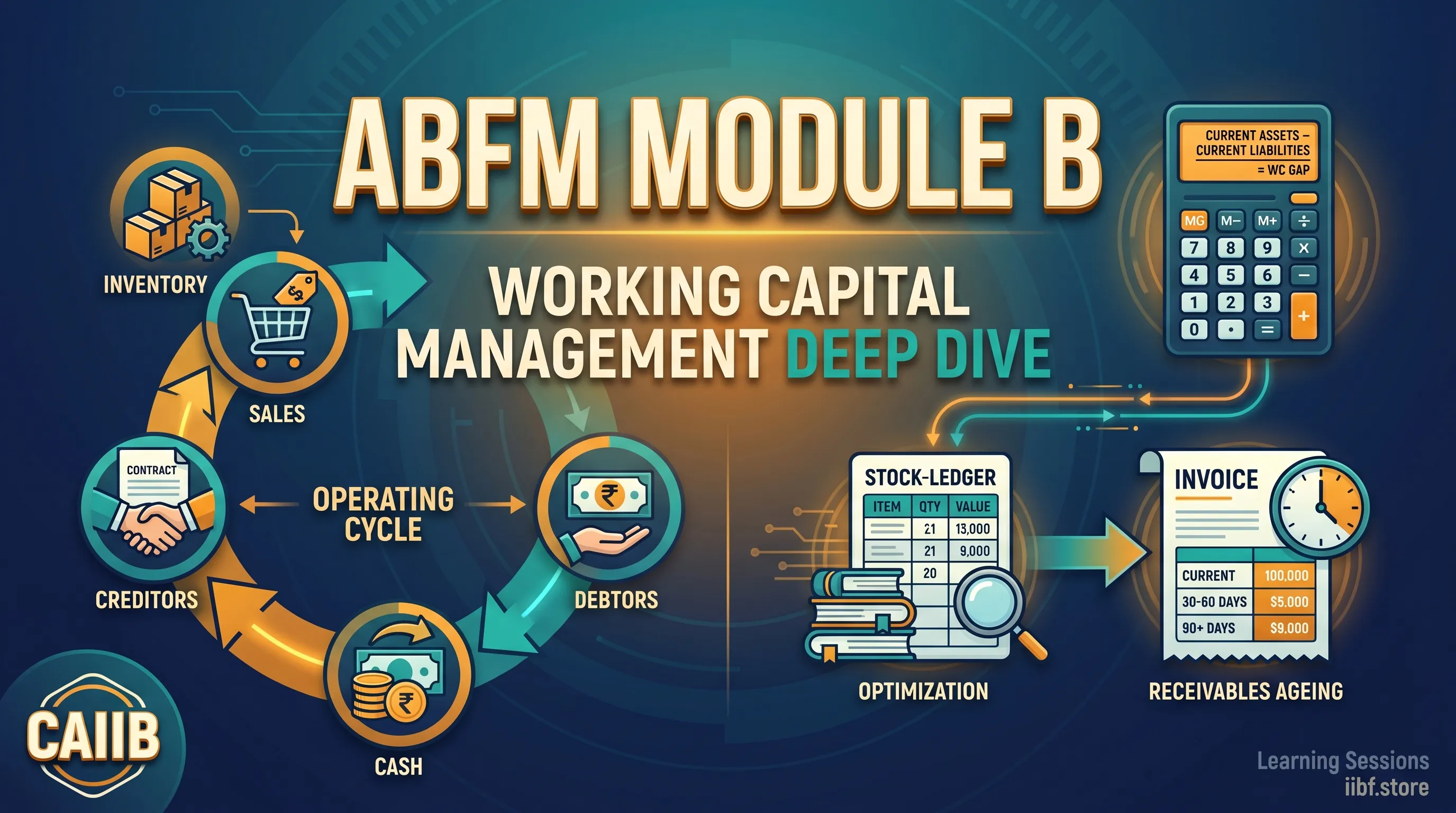
An operating cycle is the time it takes for one rupee invested in raw material to come back as cash from a customer payment. For a typical manufacturing unit:

Operating Cycle = Raw Material Holding Period + Work-in-Progress Period + Finished Goods Holding Period + Debtor Collection Period − Creditor Payment Period

Each component:

• Raw Material Holding Period = Average RM stock × 365 ÷ Annual RM consumption
• WIP Period = Average WIP × 365 ÷ Annual cost of production
• Finished Goods Period = Average FG × 365 ÷ Annual cost of goods sold
• Debtor Period = Average debtors × 365 ÷ Annual credit sales
• Creditor Period = Average creditors × 365 ÷ Annual credit purchases

Worked example: a small unit holds 30 days of raw material, takes 15 days to convert to finished goods, holds finished goods for 20 days, gets paid in 45 days, and itself pays suppliers in 30 days. Operating cycle = 30 + 15 + 20 + 45 − 30 = 80 days.

That 80-day operating cycle means the firm has 80 days of operations to fund with working capital. If annual turnover is ₹3 crore, daily turnover ≈ ₹0.82 lakh, so working capital need ≈ 80 × ₹0.82 = ₹66 lakh.

Working capital gap and MPBF methods

RBI's Tandon Committee (1974) introduced the Permissible Bank Finance (PBF) framework, refined as the Maximum Permissible Bank Finance (MPBF). Two methods (sometimes called Method I and Method II) are tested:

Method I: Bank finance = 75% of (Current Assets − Current Liabilities other than bank borrowings). The borrower contributes the remaining 25% as net working capital.

Method II: Borrower contributes 25% of total current assets as net working capital; bank finances the rest.

Method II is more conservative (higher borrower contribution). The exam loves "calculate MPBF" — drill the two formulas.

Worked example (Method II):

• Total current assets: ₹100 lakh
• Current liabilities (excluding bank borrowings): ₹20 lakh
• Working capital gap (CA − CL) = ₹80 lakh
• Borrower's contribution = 25% of CA = ₹25 lakh
• MPBF = WC Gap − Borrower Contribution = ₹80 − ₹25 = ₹55 lakh

Turnover method (Nayak Committee)

For smaller borrowers (typically up to ₹5 crore aggregate working capital limits), RBI's Nayak Committee recommended a simpler Turnover Method:

Working Capital Limit = 20% of projected annual turnover, with the borrower's contribution at 5% of turnover.

The 20% figure implies a 72-day operating cycle (since 100/72 × 14% borrower margin ≈ 20% bank finance). The method is computationally trivial — its very simplicity is why it dominates working-capital sanctions in the MSE segment.

Worked example: a small enterprise projects ₹2 crore turnover next year. Sanction limit = 20% × ₹2 crore = ₹40 lakh. Borrower contribution = 5% × ₹2 crore = ₹10 lakh. Bank finance = ₹40 lakh − ₹10 lakh = ₹30 lakh.

Cash Conversion Cycle (CCC)

CCC measures the days between when the firm pays its supplier and when it receives cash from its customer for the corresponding sale. The formula is essentially the operating cycle:

CCC = DIO + DSO − DPO

Where DIO = Days Inventory Outstanding, DSO = Days Sales Outstanding (debtor days), DPO = Days Payable Outstanding (creditor days).

Why CCC matters: a shorter CCC means faster cash turnover, lower working-capital intensity, higher ROCE. A firm with negative CCC (collects from customers before paying suppliers — common in retail like Big Bazaar / Reliance Retail) is essentially financed by its suppliers.

Inventory management techniques

Three techniques covered in ABFM Module B:

• EOQ (Economic Order Quantity) = √(2 × Annual Demand × Order Cost ÷ Carrying Cost per unit per year). The order quantity that minimises total inventory cost.
• ABC Analysis — categorises inventory items: A (high-value, tight control), B (medium-value, moderate control), C (low-value, loose control).
• VED Analysis (Vital / Essential / Desirable) — for spare parts and critical inputs in manufacturing.
• JIT (Just-in-Time) — minimal inventory, deliveries timed to production. Toyota's Kanban system is the classical example.

Receivables management

Three levers:

1. Credit policy — credit terms offered (net 30, 2/10 net 30 — i.e. 2% discount for payment within 10 days, full payment by day 30).
2. Collection policy — how aggressively follow-ups are done, when to call, when to involve the legal team.
3. Factoring / bill discounting — selling receivables to a factor at a discount to immediately monetise. Recourse vs non-recourse factoring.

The trade-off: tighter credit terms reduce DSO but may lose sales. Looser terms boost sales but stretch working capital.

Cash management

Key concepts:

• Cash budget — monthly projection of cash inflows and outflows. The basis for short-term working-capital planning.
• Float management — the difference between book cash and bank cash because of cheques in transit. Modern UPI/IMPS reduces float to near zero, but float still matters for cheque-heavy business segments.
• Baumol Model / Miller-Orr Model — optimal cash holding determination. These appear as identification questions ("which model determines optimal cash level?").
• Sweep accounts — automatic transfer of surplus cash into interest-earning instruments (and vice versa).

Exam tactics for ABFM Module B

1. Memorise the operating-cycle formula structure. Add the holding periods, subtract creditors. Plug-and-chug.
2. Drill both MPBF methods. Method I (75% of WC gap) and Method II (25% of CA borrower contribution). At least one MPBF computation appears on every ABFM paper.
3. Memorise EOQ as a formula structure. Don't worry about deriving it; the exam tests plug-and-chug.
4. Internalise the Turnover Method (20% × turnover). Simple, powerful, frequently tested.

Frequently Asked Questions

Final Word

ABFM Module B is the working-capital chapter that bridges textbook finance and your branch job. Master the operating cycle, the two MPBF methods, the Turnover Method, and the supporting techniques (EOQ, ABC, JIT, factoring) — and you've covered 30-40 marks of the ABFM paper while sharpening your credit-appraisal instincts simultaneously.

Open a free CAIIB ABFM chapter mock tonight and attempt 15 Module B questions. 65%+ on first attempt confirms readiness. Pair with our MSME credit assessment field guide for end-to-end coverage of WC-related material.

All five CAIIB papers — chapter PDFs, video classes, and timed mock tests — are free on iibf.store's CAIIB course.