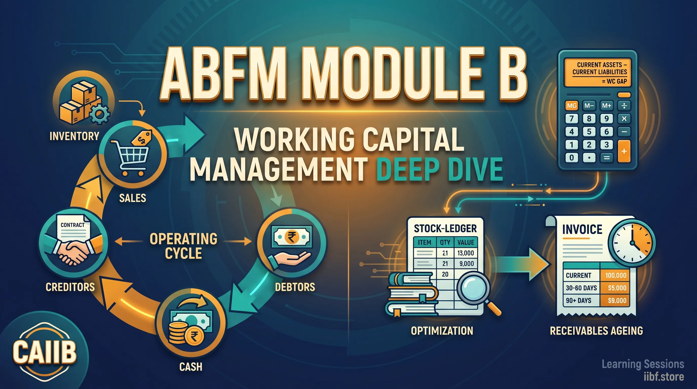
CAIIB ABFM Module B — Working Capital Management की पूरी गहराई

CAIIB का ABFM (Advanced Business and Financial Management) पेपर, और उसमें भी Module B — Working Capital Management, ज़्यादातर candidates के लिए marks बटोरने का सबसे आसान मौक़ा है। वजह यह है कि यहाँ ज़्यादातर सवाल सीधे formula-based numerical होते हैं, और ब्रांच में जो CC (Cash Credit) limits हम रोज़ sanction करते हैं, उन्हीं का theoretical version exam में आता है। आज इन्हीं concepts को step-by-step देखते हैं।

1. Operating Cycle — Working Capital की रीढ़

हर manufacturing या trading business में पैसा एक चक्र में घूमता है: कच्चा माल खरीदा → WIP में बदला → finished goods बने → बेचे गए → debtors से recovery → फिर कच्चा माल। इस पूरे चक्र की लंबाई ही Operating Cycle कहलाती है।

फॉर्मूला:

Operating Cycle (days) = RM days + WIP days + FG days + Debtor days − Creditor days

हर component अलग ratio से निकलता है — जैसे RM days = (Average RM Inventory / Annual RM Consumption) × 365। Creditor days को इसलिए घटाते हैं क्योंकि supplier ने जब तक पैसा माँगा नहीं, तब तक उतने दिन का financing वही कर रहा है। जितना लंबा cycle, उतनी ज़्यादा working capital की ज़रूरत — यही exam में बार-बार पूछा जाता है।

2. Tandon Committee की MPBF — Method I और Method II

1975 में Tandon Committee ने bank finance की norms बनाई थीं, और आज भी ABFM में यही syllabus का heart है। MPBF (Maximum Permissible Bank Finance) निकालने के दो methods हैं, और दोनों का logic समझना ज़रूरी है।

• Method I: Working Capital Gap = Current Assets (CA) − Current Liabilities other than bank borrowing (OCL)। फिर borrower को इस gap का 25% अपने पास से (margin) लाना है, बाक़ी 75% bank देगी। यानी MPBF = 0.75 × (CA − OCL)।
• Method II: यहाँ borrower का contribution बढ़ जाता है — उसे total current assets का 25% margin के रूप में लाना है। यानी MPBF = 0.75 × CA − OCL। यह method ज़्यादा conservative है क्योंकि current ratio automatically 1.33 हो जाता है।

परीक्षा का shortcut: एक ही data पर दोनों methods लगाएँ तो Method II हमेशा कम MPBF देगा। RBI ने धीरे-धीरे Method II को preferred बनाया, और बड़े borrowers के लिए Method III (Core Current Assets long-term finance से) भी सुझाया था — हालाँकि practice में Method II ही चलता है।

3. Nayak Committee Turnover Method — छोटे borrowers के लिए

1991 में Nayak Committee ने SSI और छोटे units के लिए simplified approach दिया, जो आज भी ₹5 crore तक की limit वाले MSME borrowers पर लागू है। Logic यह है कि छोटे units पर detailed CMA data माँगना practical नहीं।

नियम सीधा है:

• Total Working Capital requirement = projected annual turnover का 25% (मान लिया गया कि operating cycle 3 महीने है)।
• इसमें से borrower को 5% अपनी margin लानी है।
• Bank की limit = projected turnover का 20%।

उदाहरण: अगर projected turnover ₹4 करोड़ है, तो bank की WC limit = ₹80 लाख, और borrower का contribution ₹20 लाख। यही method ब्रांच में हम MSME borrowers को CC limit देते वक़्त रोज़ use करते हैं — MUDRA और छोटे लोन के सिलसिले में यह पूरा flow इस article में देख सकते हैं।

4. Cash Conversion Cycle (CCC) — Modern नज़रिया

Operating Cycle से एक कदम आगे है CCC, जो बताता है कि कंपनी का पैसा कितने दिन inventory और receivables में फँसा रहता है, suppliers का credit काटने के बाद।

CCC = DIO + DSO − DPO

जहाँ DIO = Days Inventory Outstanding, DSO = Days Sales Outstanding, और DPO = Days Payable Outstanding। जितना छोटा CCC, उतना efficient business — Amazon और Walmart जैसी companies का CCC तो negative भी होता है, यानी customer से पैसा पहले आ जाता है, supplier को बाद में देते हैं।

5. Inventory Management — EOQ का famous formula

कितनी quantity एक बार में order करें ताकि ordering cost और carrying cost दोनों minimum हों? इसी का जवाब है Economic Order Quantity (EOQ):

EOQ = √(2DA / H)

जहाँ D = annual demand, A = ordering cost per order, H = holding cost per unit per year। साथ में तीन और तकनीकें ज़रूर याद रखें:

• ABC Analysis: Value के हिसाब से inventory को A (high), B (medium), C (low) में बाँटना — A items पर सख़्त control।
• VED Analysis: Criticality के हिसाब से — Vital, Essential, Desirable। ज़्यादातर hospitals और defence में।
• JIT (Just-in-Time): Inventory लगभग शून्य रखना, supplier से माँग पर delivery। Toyota का famous system।

6. Receivables और Cash Management

Receivables side पर तीन lever हैं: credit policy (किसको कितने दिन का credit), collection efforts, और factoring (receivables को factor company को discount पर बेच देना)। Cash management में दो classical models पूछे जाते हैं:

• Baumol Model: Cash को inventory की तरह treat करता है — optimum cash balance = √(2 × T × F / i), जहाँ T = total cash need, F = transaction cost, i = interest rate। मानता है कि cash usage steady है।
• Miller-Orr Model: Real-world ज़्यादा random है — यह upper और lower limit set करता है, और cash उससे बाहर जाए तब transaction होता है। ज़्यादा practical।

परीक्षा रणनीति

Module B में numerical सीधे formulas पर आते हैं — operating cycle days, MPBF दोनों methods, Nayak का 20%, EOQ का square root। Theory से ज़्यादा practice ज़रूरी है। iibf.store/tests पर ABFM Module B के chapter-wise mock tests उपलब्ध हैं, और structured तैयारी के लिए पूरा CAIIB course यहाँ देखें।