Value at Risk Calculation Methods for Bank Risk Management
Every bank risk manager eventually has to answer one question in plain numbers: how much can we lose tomorrow if markets move against us? That is exactly what Value at Risk calculation methods are built to answer, and IIBF's Risk Management paper expects candidates to know not just the definition but how each method is actually computed, where it works, and where it quietly fails. This article walks through the three standard approaches banks use, how the holding period and confidence level are chosen, how VaR sits inside the Basel capital framework, and the limitations examiners love to test. If you are preparing for the standalone Risk Management certification, treat this as the practical bridge between the textbook formula and how a treasury desk actually reports risk every morning.
📊 What Is Value at Risk and Why Banks Use It
Value at Risk (VaR) is a statistical estimate of the maximum loss a portfolio could suffer over a given holding period, at a given confidence level, under normal market conditions. A bank reporting a one-day VaR of Rs 5 crore at 99% confidence is saying: on 99 out of 100 trading days, the loss on this book should not exceed Rs 5 crore. It says nothing about the remaining 1% — that is exactly where stress testing takes over.
Banks use VaR because it compresses a portfolio's exposure to interest rates, equity prices, exchange rates, and credit spreads into a single rupee number that a board can understand without reading a Greeks table. It is used to set trading limits, allocate capital, and report market risk under the RBI's capital adequacy framework. But a single number is only as good as the method used to build it, and that is where the three calculation methods diverge.
🧮 The Three Value at Risk Calculation Methods
The historical simulation method revalues today's portfolio using actual price changes observed over a past window — typically 250 to 500 trading days — and reads off the loss at the required percentile. It needs no assumption about the shape of the return distribution, which is its biggest strength, but it is only as good as the historical window: a quiet twelve months will understate tail risk.
The variance-covariance (parametric) method assumes portfolio returns are normally distributed and calculates VaR directly from the portfolio's volatility and correlation matrix. It is fast to compute and works well for portfolios of linear instruments like plain bonds and equities, but it badly underestimates risk for portfolios loaded with options, because it cannot capture non-linear payoffs or fat tails.
The third approach, covered in depth in our companion piece on Monte Carlo simulation in risk management, generates thousands of random price paths from a specified statistical model and revalues the portfolio under each one. It handles non-linear instruments and complex derivatives better than the other two methods but is the most computationally expensive and depends heavily on the model chosen to generate the scenarios.
💡 Exam Tip: If a question asks which method best captures option non-linearity, the answer is Monte Carlo simulation, not the variance-covariance method — this is a favourite trap in IIBF Risk Management papers.

⏱️ Choosing the Holding Period and Confidence Level
Two inputs decide how conservative a VaR number is: the holding period and the confidence level. A longer holding period assumes the position cannot be exited quickly, so illiquid instruments demand a longer period than a liquid government security. Banking regulators historically anchored market risk capital charges to a 10-day holding period, while trading desks often monitor a 1-day VaR for daily limit management and simply scale it up for regulatory reporting.
The confidence level — usually 95% or 99% — sets how far into the tail the estimate reaches. A 99% VaR is always larger than a 95% VaR on the same book, because it is reserving for a rarer, worse outcome. Raising the confidence level does not make the portfolio safer; it only changes how much of the loss distribution the reported number is designed to cover.
Candidates preparing chapters on regulatory capital and capital adequacy should note that the assumptions feeding VaR — holding period, confidence level, and lookback window — are themselves risk management decisions, not fixed constants, and IIBF questions often test whether you understand this trade-off rather than just the formula.
🏦 VaR Under the Basel and RBI Capital Framework
Under the Basel market risk framework, banks that meet the eligibility criteria can use an internal VaR-based model to compute regulatory capital for their trading book, subject to supervisory approval and ongoing validation by the Reserve Bank of India. Banks that do not qualify fall back on the simpler standardised approach. This choice, and the supervisory scrutiny that comes with it, is assessed through the supervisory review and evaluation process under Basel Pillar 2, which examines whether a bank's internal risk models are actually fit for the risks it is running.
None of this exists in isolation from why the framework was built in the first place. Understanding why banks need regulation gives context for why VaR-based capital charges exist at all — to make sure a bank's own capital cushion is sized to the risk it is actually carrying, not just to what it reports on a good quarter. For current repo, reverse repo and policy rate context that feeds into interest rate VaR calculations, keep an eye on the RBI rates resource page.
⚠️ Common Mistake: Students often assume VaR models are only for market risk. In practice, VaR-style thinking also informs credit risk economic capital models and, more broadly, sits inside the wider enterprise view alongside operational risk and management framework — do not treat these as unrelated silos in the exam.

⚠️ The Limitations of VaR
VaR has three well-documented weaknesses that IIBF loves to probe. First, it says nothing about the size of losses beyond the confidence level — two portfolios can have identical 99% VaR while one has a far worse tail because it is not a coherent risk measure in the technical sense. Second, VaR built on historical data assumes the future will resemble the past, which fails precisely during a crisis, when correlations between asset classes spike and historical relationships break down.
Third, VaR is a static snapshot; it does not tell a bank how a position would behave under a specific extreme scenario, such as a sudden sovereign downgrade or a sharp currency depreciation. This is exactly why VaR is never used alone — it is paired with stress testing and scenario analysis, and governance structures such as the three lines of defense model exist to make sure model outputs like VaR are independently reviewed rather than taken at face value by the desk that generates them.
📌 Remember: VaR answers "how much could I lose on a normal bad day," not "how much could I lose on the worst day." Confusing the two is the single most common conceptual error in this topic.
🎯 VaR in the Bigger Risk Management Picture
Market risk measured through VaR is only one slice of a bank's overall risk profile. Credit losses that materialise when a corporate borrower defaults follow an entirely different track — including formal insolvency steps such as an operational creditor demand notice under the Insolvency and Bankruptcy Code, which is a recovery mechanism, not a market risk tool, but ultimately feeds back into the same capital adequacy calculations that VaR-based charges also affect.
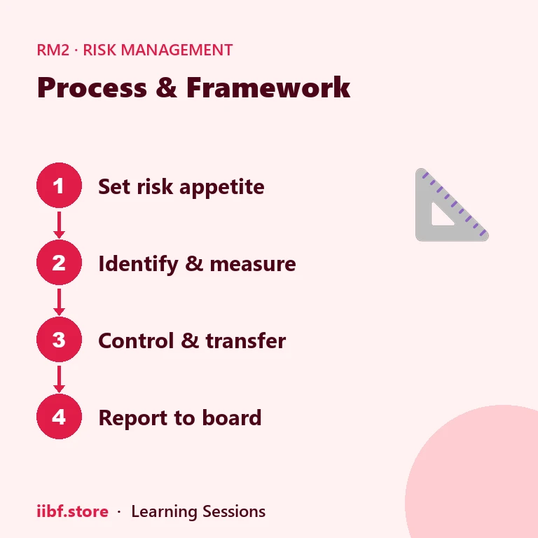
A well-run risk management function does not treat market, credit, and operational risk as separate departments reporting separately upward. It aggregates them, tests them against common stress scenarios, and reports a consolidated picture to the board. That integration, and the technology and governance layers that support it, are worth revisiting through our broader risk management article series before exam day.
| Method | Distribution Assumption | Handles Options Well | Computation Speed |
|---|---|---|---|
| Historical Simulation | None (uses actual past returns) | ✅ Partially | Moderate |
| Variance-Covariance | Normal distribution assumed | ❌ No | Fast |
| Monte Carlo Simulation | Model-defined | ✅ Yes | Slow |
🧠 Practice MCQs: Value at Risk Calculation Methods
Q1. Which VaR method assumes portfolio returns follow a normal distribution? (a) Historical simulation (b) Variance-covariance method (c) Monte Carlo simulation (d) Stress testing
Answer: (b) — The variance-covariance (parametric) method relies on a normal distribution assumption and the portfolio's volatility-correlation matrix.
Q2. A 99% one-day VaR of Rs 5 crore means: (a) The maximum possible loss is Rs 5 crore (b) The loss will never exceed Rs 5 crore (c) On 99 out of 100 days, the loss should not exceed Rs 5 crore (d) The average daily loss is Rs 5 crore
Answer: (c) — VaR is a probabilistic statement at a given confidence level, not an absolute ceiling on loss.
Q3. Which VaR method best captures the non-linear payoff of options? (a) Variance-covariance method (b) Historical simulation only (c) Monte Carlo simulation (d) None of the methods can
Answer: (c) — Monte Carlo simulation revalues the portfolio across many simulated paths, capturing non-linear option payoffs that the parametric method misses.
Q4. What is the main limitation of VaR as a risk measure? (a) It is too expensive to calculate (b) It does not indicate the severity of losses beyond the confidence level (c) It cannot be used for market risk (d) It requires no historical data
Answer: (b) — VaR is silent on tail severity beyond the chosen confidence level, which is why it is supplemented with stress testing.
Q5. Under the Basel market risk framework, which approach can eligible banks use as an alternative to the standardised approach? (a) Internal VaR-based model, subject to supervisory approval (b) Fixed percentage of gross income (c) Loss distribution approach only (d) Basic indicator approach
Answer: (a) — Banks meeting supervisory criteria can use approved internal VaR-based models for market risk capital instead of the standardised approach.
Want chapter-wise mock tests with 100+ MCQs? Start practising free →
Frequently Asked Questions
What is the difference between VaR and stress testing?
VaR estimates the loss expected under normal market conditions at a chosen confidence level, while stress testing measures the loss under a specific, deliberately severe scenario that VaR does not cover. Banks use both together, not as substitutes.
Which VaR method is most commonly used by Indian banks for regulatory reporting?
Most banks use a combination — the historical simulation or variance-covariance method for routine daily reporting because they are computationally light, and Monte Carlo simulation for books with significant options or structured products where non-linear risk must be captured accurately.
Does a higher confidence level make a bank's VaR estimate more accurate?
No. A higher confidence level, such as 99% instead of 95%, simply reserves for a rarer and larger loss; it does not improve the accuracy of the underlying model or data. Model quality and data length matter more than the chosen confidence level.
Is VaR relevant outside market risk in the IIBF Risk Management syllabus?
The concept underlies economic capital calculations across risk types, including credit risk, and ties into the broader enterprise risk view examined alongside operational risk, governance, and regulatory capital chapters in the syllabus.
Value at Risk calculation methods are one of the most testable, practical topics in the entire Risk Management syllabus because they combine statistics, regulation, and real trading-desk practice in one place. Revise the three methods side by side, know their limitations cold, and work through timed practice questions on the IIBF Risk Management mock test series to make sure the concepts hold up under exam pressure.
Practice this topic
Take a free mock test, download chapter PDFs, or watch a video class — all included on iibf.store.
Keep reading